Science
Gravitational Waves & Universe Sandbox ²
Feb 15th
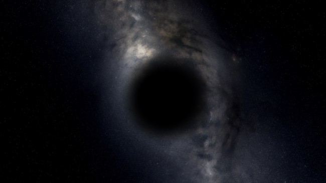
A black hole in Universe Sandbox ². Researchers concluded the detected gravitational waves resulted from two black holes colliding.
What’s the significance of discovering gravitational waves?
This announcement is a huge deal. It is on par with the discovery of the Higgs Boson particle which provided the missing evidence for a prediction of the Standard Model of particle physics. Gravitational waves are a century-old (almost exactly) prediction now confirmed by a huge number of relentless, and brilliant people after many years of hard work. It is the first direct confirmation of the prediction from Einstein’s General Relativity that matter and energy determine the motion of bodies by warping the fabric of spacetime itself, and in so doing, emanate ripples when massive bodies are accelerated through that space.
It is not only confirmation of general relativity, though. It is also the first of many future observations that will look at the universe in a completely new way. Up until now we’ve used only photons (telescopes all along the electromagnetic spectrum) and sometimes neutrinos. Now we can add listening to the fabric of space to our list of tools. This will allow us to see the dark and the obscured parts of the universe: the early universe, centers of galaxies, things blocked by dust clouds, and so on, by listening for changes in space itself. It is the start of a new age in astronomy.
In addition to this detection being the first direct proof that the predictions of general relativity that matter and energy warp space time are true, and some of the strongest evidence for the reality of black holes, this is also a new kind of astronomy. Though gravity is the weakest force and gravitational waves are very hard to detect, they do have a few advantages over observations of photons.
- First, gravitational waves are practically impervious to matter in their path. This means we can see into regions of space that are blocked to optical observatories, such as inside dense clouds of dust, the centers of galaxies, behind large or close bodies.
- Second, this is an observation of the warping of space itself, meaning we can detect things that have mass but might not produce observable light, such as black holes, dense sources of dark matter (if such were to exist), cosmic string breaks, etc.
- Third, gravitational waves fall off in amplitude much more slowly than light. This means that we can receive signals from very far away that we might not notice optically.
- And fourth, because gravitational waves also travel at the speed of light and don’t have to bounce off intervening matter, and begin to be potentially detectable from bodies getting close rather than just after the moment of collision, this means that we can work with other telescopes and tell them “Look over there! You’re probably going to see something exciting!”
This all of means that this detection means the beginning of a new kind of observational astronomy, as well as a better understanding of of of the fundamental forces of the universe, gravity.
What role did Jenn, astrophysicist and Universe Sandbox ² developer, play in the discovery?
While I was in the field I ran super-computer simulations to make predictions about the gravitational wave signals that would be produced by binary black hole mergers. Those waveforms are used as templates in the detector pipeline. The detector matches the template banks against the incoming data to find real signals amidst the noise of the detector, while also doing searches for large burst signals (how this one was found). Those waveforms are then used again to determine where the signal came from, what it was (two black holes, a neutron star and a black hole, two neutron stars, etc), and the properties of the bodies that created the signal (spins, masses, separation, etc.). I also worked on developing the analytical formulas to determine those spins and masses from those signals.
Here’s one of the scientific papers on the process of determining the properties of the source of the signal, with three papers cited on which Jenn Seiler was an author:
https://dcc.ligo.org/public/0122/P1500218/012/GW150914_parameter_estimation_v13.pdf
The Einstein equations for general relativity are ten highly non-linear partial differential equations. This means that it is only possible to obtain exact solutions for astrophysical situations for some very idealized conditions (such as spherical symmetry and a single body). In order to predict the gravitational waveforms produced by compact multi-body systems, or stellar collapse, it is necessary to solve the equations numerically (computationally). This means formulating initial data for spacetimes of interest (such as two in-spiralling black holes of various spins and mass ratios) and evolving them by integrating the solutions of the Einstein equations stepping forward in time by discrete steps. To prove that these computer simulations approximate reality more than just by equations on paper we would run these simulations at multiple resolutions for our discrete spacetimes and show that our solutions converged to a single solution as we approach infinite resolution (that would represent real continuous space) at the rate we expect for the method we were using.
There were many obstacles in creating these simulations: vast amounts of computational power required for accuracy; the fact that we needed to run tons of these large, slow, computationally intensive simulations in order to cover the parameter space (spins, masses, orientations, etc) of potential sources of gravitational waves; and so on. For black holes, one major challenge was the fact that they contain a singularity. A singularity means an infinity, and computers don’t like to simulate infinities. Numerical relativity researchers had to find a way to simulate black holes without having the singularity point in the slicing of the spacetime integrated in the simulation. The first successful simulation of this kind didn’t happen until 2005 (http://journals.aps.org/prl/abstract/10.1103/PhysRevLett.95.121101).
Once we had working simulations, groups around the world set to work on simulating the gamut of major potential gravitational wave signal sources. These simulation results were not just useful to the detectors to help identify signals, but also to the theorists to help formulate predictions about the results of such astrophysical events. Predictions such as: the resulting velocity of merged black holes from binaries of various spins, the amount of energy released by black hole mergers, the effect that black hole spins have on the spins and orbits of other bodies, etc.
When will you add gravitational waves into Universe Sandbox ²?
We really can’t do gravitational waves in an n-body simulation, which is the method Universe Sandbox ² uses to simulate gravity. N-body simulations look at the effect that each body has on each other body in a system at small discrete time steps.
General relativity requires simulating the spacetime itself. That is, taking your simulation space, discretizing it to a hi-res 3-D grid and checking the effect that each and every point in that grid has on all neighboring points at every timestep. Instead of simulating N number of bodies, you are simulating a huge number of points. You start with some initial data of the shape of your spacetime and then see how it evolves according to the Einstein equations, which are 10 highly non-linear partial differential equations. Accurate general relativity simulations require supercomputers.
There are some effects and features related to relativity that would be possible to add to Universe Sandbox ², however. Here are a few we are discussing:
-
Gravity travelling at the speed of light.
-
Currently if you delete a body in a simulation, the paths of all other bodies instantly respond to the change. The reality is that it would not be instantaneous; it would take time for that information about the altered gravitational landscape to reach a distant object.
-
-
Spinning black holes.
-
Most black holes are very highly spinning. If you imagine a spinning star collapsing it is easy to understand why. This is the same effect as when a spinning figure skater pulls in their arms; because of conservation of angular momentum, they spin faster. A consequence of this spin is that, while the event horizon would remain spherical, there would be an oblate spheroid (squished ball) around the black hole called an ergosphere. This ergosphere twists up the spacetime contained within it and accelerates bodies that enter this region (as well as affecting their spins). Because it is outside of the event horizon, this means one can slingshot away from this region and even steal energy from the rotation of that black hole.
-
-
Corrections to the motions of bodies to approximate general relativity.
-
Loss of momentum due to the emission of gravitational waves causes close massive bodies to inspiral. With this you could recreate the decaying orbits of binary pulsars.
-
Spins of close bodies affect each other’s motion and spins (see above). This would give you things like spun up accretion disks around black holes.
-
These corrections would be made by adding post-newtonian corrections to body velocities.
-
Learn more
Bad Astronomy article: LIGO Sees First Ever Gravitational Waves as Two Black Holes Eat Each Other
Video and Comic Explaining Gravitational Waves
Reddit AMA (Ask Me Anything) by LIGO Scientists
Paper by LIGO Researchers: Observation of Gravitational Waves from a Binary Black Hole Merger
Alpha 18.2 | Planet Nine | Now Available
Jan 21st
Planet Nine
The discovery of a hypothetical ninth planet in our solar system was announced on January 20th, 2016 by researchers at the California Institute of Technology.
Universe Sandbox ² Alpha 18.2 features two simulations of Planet Nine. Run Steam to update, then check them out in Home -> Open -> Possible Planet Nine [and] Evidence of a Ninth Planet.
Or buy now for instant access to Universe Sandbox ² on Steam Early Access:
http://store.steampowered.com/app/230290/
The announcement comes after years of research into explaining the peculiar, but very similar, orbits of six small bodies orbiting beyond Neptune. Many theories have been proposed, but none has been as compelling as a very distant ninth planet pulling these bodies into their highly elliptical orbits. Using mathematical modeling, the two researchers, Konstantin Batygin and Mike Brown, have shown that a ninth planet fits very well into the data we have about objects in the Kuiper Belt and beyond.
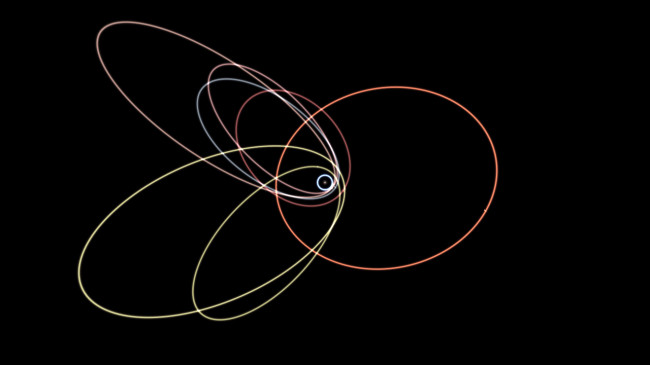
There’s only a 1 in 15,000 chance that the clustering of the orbits on the left is coincidental. Another explanation is the gravitational influence of a ninth planet, whose orbit is represented by the yellow line on the right. (from Universe Sandbox ²)
Planet Nine has not been directly observed yet by telescope, which is why it is hypothetical. But the researchers say there is a very good chance of spotting it in the next five years. It is suspected to be about 10 times the mass of Earth, similar in size to Neptune, with an orbit that’ll take it around the Sun every 10,000 – 20,000 years.
Of course, we don’t know how Planet Nine got there. Brown and Batygin propose that this planet was formed in the early days of the solar system, along with Jupiter, Saturn, Uranus, and Neptune. Then it could have been shot outward by one of the gas giants, and instead of leaving the solar system entirely, it may have been slowed down by gas in the Sun’s protoplanetary disk, enough to keep it in orbit.
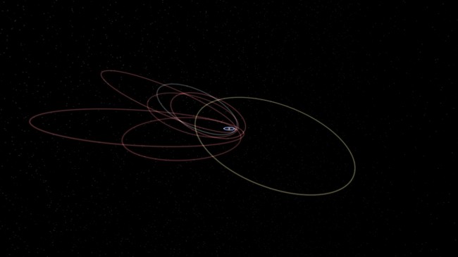
Alternative angle of Planet Nine (yellow orbital line) and the six objects used in the analysis. (from Universe Sandbox ²)
If the ninth planet does exist, then it will be the second time our solar system will have claim to nine planets… After, of course, Pluto was demoted in 2006. But Brown says there’s no question that the hypothetical ninth planet is indeed a planet. It’s likely much bigger than Earth, and has a large influence on other bodies in the solar system. And besides, Brown would know — his discovery of Eris was the reason Pluto was voted out.
Here’s a great discussion of Planet Nine by Mike Merrifield, an astronomer and professor at the University of Nottingham:
We’re hope you’re as excited about this possible discovery as we are! Make sure you check out the new simulations in Universe Sandbox ²: Home -> Open -> Possible Planet Nine [and] Evidence of a Ninth Planet.
See the complete list of What’s New in Alpha 18.2: What’s New
Additional links about Planet Nine:
Astronomers say a Neptune-sized planet lurks beyond Pluto
Evidence grows for giant planet on fringes of Solar System
Evidence for a Distant Giant Planet in the Solar System (research paper)
Simulating the World of Game of Thrones in Universe Sandbox ²
Jul 17th
An Unpredictably Long Winter is Coming
Fans of George R. R. Martin’s fantasy series A Song of Ice and Fire or the television series, Game of Thrones, know well the often repeated warning, “Winter is coming.”
For those living on the continent of Westeros in this fantasy world, summers can be long, and so can the winters. But some winters are especially cold and last for several years, while others are relatively mild and short.
What causes this variance in seasons? Martin doesn’t offer an explanation, so we’re free to speculate.
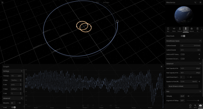
One research paper (“Winter is coming”) proposes that perhaps there’s a natural explanation: Westeros is on a circumbinary planet, meaning its orbit extends around a binary star system.
Simulating Westeros in Universe Sandbox ²
The paper may be tongue-in-cheek, but that doesn’t mean we can’t use its parameters to try simulating it in Universe Sandbox ². Like the paper, we were unable to find stable orbital parameters that would create the level of unpredictability discussed in the books or the show.
We could, however, create a system that has variable winter and summer intensities on regular predictable intervals with a large northern polar ice region. Though our results didn’t exactly match those in the paper, we managed to recreate similar seasonal patterns to what the authors describe in their paper.
If you own Universe Sandbox ², you can see this simulation for yourself in Alpha 15: Home -> Open -> Fiction -> Lands of Ice & Fire | Game of Thrones.
To open the temperature graph, open the Westeros planet’s Properties, select the Climate tab, hover over the Surface Temperature icon and click the Graph button.
If you don’t own Universe Sandbox ², you can buy it now to get instant access to the alpha via Steam code: http://universesandbox.com/2
Happy Earth Day!
Apr 22nd
First observed in 1970, Earth Day now gathers over 1 billion people in 192 countries every year on April 22 to celebrate our planet and raise awareness of the issues it faces. According to Earth Day Network, that makes it the largest civic observance in the world.
The growth of this movement toward the care and appreciation for our planet is evident all around us. Environmental awareness is no longer reserved for activists and radicals. “Going green” and “reducing your footprint” have become familiar, if not trendy, concepts.
But despite this, human-caused climate change continues to take us further down the road toward inevitable crisis. It’s a bleak forecast, but one that we, as individuals, nations, and a global community, must confront if we want to create the necessary changes.
Earth in Universe Sandbox ²
In Universe Sandbox ², we’ve added a simple climate simulation for Earth. We hope it helps in understanding how our climate works, and how fragile our planet is.
Here are a few things you can try in Universe Sandbox ²:
-
Simulate Future Climate Scenarios
- We’ve included the ability to simulate scenarios based on data from the most recent IPCC report
- We recommend trying the Climate Scenarios activity (Home -> Main tab)
- You’ll learn how to use the different models and graph Earth’s temperature over time
- Learn more about simulating these scenarios in our previous blog post
-
Tidally lock the Earth to the Sun
- Select Earth (in the default Solar System sim)
- In Earth’s properties window, click the “Motion” tab
- Scroll down and click “Tidally Lock”
- Now one side of the planet will always face the Sun
- And the other side of the planet will begin to freeze over
- Tidal locking is why there’s a “dark side of the moon.” From here on Earth, we can only ever see the same side
-
Turn Earth into a Comet or a Snowball
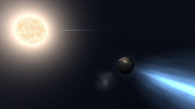
- Try moving the Earth closer to the sun to turn it into a comet.
- Or move the Earth out past Mars and watch it freeze over. (Load the sim “Earths Next to Sun” to see multiple Earths at various distances from the Sun)
If you don’t own Universe Sandbox ², you can get instant access to the alpha through our website: universesandbox.com/2
Future Earth Climate Scenarios
Feb 20th
One of the most important features in Universe Sandbox ² is the ability to simulate Earth’s climate. It’s a relatively simple simulation, but it helps demonstrate exactly how fragile and ever-changing our climate is.
In Alpha 13, you can select possible future scenarios for Earth’s climate. These scenarios simulate the rise in carbon dioxide levels in Earth’s atmosphere caused by human activity up until the year 2100.
To simulate these, we use the same Representative Concentration Pathways used in the latest report from the Intergovernmental Panel on Climate Change (IPCC). These four pathways are projections for the future of greenhouse gas emissions and resulting concentrations in our atmosphere. You can see each pathway’s projections in the graphs below (left: emissions; right: concentration).

CO₂ emissions and associated concentrations generated from the RCP Database.
There are many factors we can consider when looking at what changes will affect emissions. Policies, land use, global population, our attitudes toward production and consumption — these can all have a huge impact on greenhouse gas emissions. Each RCP makes different assumptions about how and when these factors might change.
To stabilize concentrations, decreases in emissions are required, because even when emissions are lowered, CO₂ hangs around in the atmosphere for a long time.
Not only do the scenarios project different outcomes for concentrations, but, importantly, they each follow a unique trajectory based on a range of possible socio-economic changes. One assumes a peak in greenhouse gases in the next decade, while another assumes that there will never be stabilization. (This is simplified for the sake of this introduction; you can learn more here.)
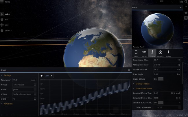
In Universe Sandbox ², you can enable RCPs by selecting the Climate tab in Earth’s properties and toggling “Select an RCP Scenario.” The default is RCP 8 5. Click the (+) icon to select one of the other 4 scenarios.
Once enabled, the pathway’s concentration level will be tied to the simulation year. The change in net radiative energy balance is also specified by the scenarios, and we put that right into our energy balance as a decrease in outgoing infrared energy. This has the effect of increasing the greenhouse effect and ultimately increases the average temperature of the planet. To see how the different scenarios play out, you can graph Earth’s temperature over the course of several decades. Below is a simulation of RCP6 through 2100.
These pathways are not forecasts. But simulating them in Universe Sandbox ² can help you gain a more intuitive understanding of what is possible for the future of Earth’s climate.
Check out this blog post by Naomi, Universe Sandbox ²’s climate scientist, to learn more about how we simulate climate: Climate in Universe Sandbox ².
You can also check out the climate tutorials right in Universe Sandbox ²: Home -> Main -> Activities.
Watch a Demo of Atmospheric Scattering
Jan 23rd
In this video, Chad, our technical artist, demos his recent work on shaders which simulate atmospheric scattering (in real-time, of course).
Atmospheric scattering is a process in which particles in a planet’s atmosphere scatter sunlight. It is the reason why the sky is blue, and why the setting sun is red.
https://www.youtube.com/watch?v=6gfFPfgovoY
Please note: This video is a demo created by Chad; it is not from Universe Sandbox ². Atmospheric scattering is an experimental feature still in its early stages. Do not expect to see this implemented in an alpha release anytime too soon.
More information on atmospheric scattering:
If you do not yet own Universe Sandbox ², you can buy it now to get instant access to the alpha, as well as free updates up to and including the final release: universesandbox.com/2.
Black Hole Rings in Universe Sandbox ²
Jan 13th
Have you seen Interstellar? Without revealing too much of the plot… the sci-fi film follows a group of astronauts who search the depths of space in hopes of finding a new home for the human race.
The film’s special effects team worked with astrophysicist Kip Thorne in order to create visual effects that were not only beautiful representations of our universe, but were also founded on accurate science (Wired article).
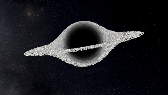
One phenomenon they wanted to simulate was a massive black hole with an accretion disk. What they ended up with is certainly impressive: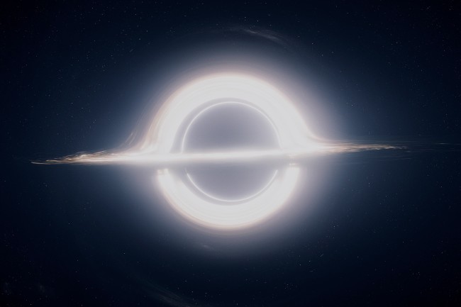
Turns out, if you add rings to a black hole in Universe Sandbox ², you get something that looks pretty similar:
Of course, you’ll notice a few differences between these images. But that might be because the first image is from a pre-rendered animation made for a film with a $165 million budget, and the second is from a real-time, interactive simulation that can run on your home computer.
If you don’t yet own Universe Sandbox ², buy it now to get instant access to the Alpha through Steam as well as free updates up to and including the final release: universesandbox.com/2
Watch a Demo of Exoplanet Detection in Universe Sandbox ²
Dec 9th
The video below was created by Eric, an astronomer working on Universe Sandbox ².
He explains how we calculate both radial velocity and normalized light curves, two key components in methods of detecting exoplanets.
You will be able to try out these new features for yourself in an upcoming alpha of Universe Sandbox ².
If you do not yet own Universe Sandbox ², you can buy it now to get instant access to the alpha, as well as free updates up to and including the final release: universesandbox.com/2.
Climate in Universe Sandbox
Oct 10th
We’ve added a simple climate simulation to the Earth in Universe Sandbox. In doing so we wanted something that would give us different temperatures at different latitudes, so we could show the seasons come and go. Where it’s cold enough for snow and sea ice, we paint the Earth white.
We also needed something simple enough that we could do the calculations in real time. And we wanted something in the spirit of the sandbox, so that you can change other things about the simulation and see the interactions play out. So we needed to respond to changes in the orbit, to incoming star-light, and even let you play around with some of the model parameters themselves.
Finally we wanted to representatively illustrate the effect of Greenhouse gases in the atmosphere, including the changes in temperature that happen when we add more Greenhouse gases to the atmosphere due to human activities. What follows is the working documentation for this feature, and should help answer some of the questions you may have. See also the evolving FAQ.
– Naomi, and the rest of the Universe Sandbox team
Balancing Energy to Calculate Temperature
The energy balance of a planet determines the temperature at the surface. What is a planetary energy balance? The amount of energy coming in from the local sun is balanced by the outgoing energy emitted in the infrared. The hotter an object the more it emits in the infrared. One can set up an energy balance equation and solve it for the surface temperature.
In the simplest version it also depends on the albedo (or reflectivity): the amount of incoming energy from the star that is reflected back instead of absorbed. You can also specify the fraction of outgoing infrared energy that gets absorbed and re-emitted towards the surface by the atmosphere on the way out.
We know that the greenhouse effect keeps the Earth a bit over 30 degrees warmer than what it would be without an atmosphere at all, which is a lot in terms of global average temperature. Even a one or two degree change in global average temperature can involve major changes to the climate.
Planets in Universe Sandbox ² have this simple global average energy balance to determine their temperature. You can change the albedo, or see what happens when you move the planet closer to or farther from the nearby star(s). For Earth (and soon Mars) we do something a bit more complicated.
Earth is Frozen at the Poles
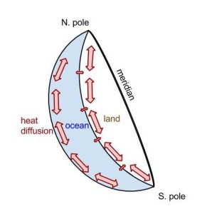
Knowing global average temperature is not enough information to determine where it’s cold enough for snow and sea ice to form and where it’s not, and when. If we did the energy balance of each latitude independently, we wouldn’t get it right. The equator would be too warm. The poles would be too cold and have much larger temperature swings with the seasons than actually occur. The reason that the equator and poles aren’t more different in temperature is because the atmosphere and the ocean redistribute energy between the equator and the poles (or meridionally, for along-meridians of North-South lines of longitude).
To do a detailed simulation of equator-pole heat redistribution you’d need a General Circulation Model (or Global Climate Model, GCM), because heat is actually transferred via large-scale circulation of air and ocean water in three dimensions. This would be way too much number-crunching to do on your computer in real-time [1].
 Luckily we can use a simpler model that was popular in the 1970s before computers were quite so powerful, and which is still used to explore basic concepts about the climate. This meridional energy balance model gives us not just a global average surface temperature, but different temperatures at each of a fixed number of latitudes[2]. This model still balances the incoming and outgoing energy globally, but also transfers energy between equator and pole, represented mathematically as a one-dimensional diffusion.
We use a version that gives us two related equations to solve: one for temperature over land, and one for the ocean. Then we do some fancy number-crunching to determine all the temperatures at all the latitudes simultaneously.
Why is this all necessary?
Without doing a simulation as complicated as this one we could never capture the seasons! Sure we could just make a game that shows you the seasons coming and going without actually calculating all these temperatures, but then it wouldn’t react correctly if you changed the tilt or the orbit of the Earth, and this is a sandbox afterall. We’re always finding the current amount of incoming starlight at each latitude depending on the luminosity of the star, its distance to the Earth, and which latitudes are getting hit with more solar energy on a given day because of Earth’s tilt.
You can also understand one of the self-reinforcing cycles that amplifies changes in the climate. When it gets colder more snow and ice forms, and when there’s more snow and ice the Earth as a whole is more reflective of incoming light. More reflection means less energy coming into the Earth system, which means it gets even colder and more snow and ice forms, and so on. The opposite can happen as well. Thus you’ll see if you move the Earth away from the Sun and freeze it over that you can’t just move it back to where it was before to unfreeze it. You have to move it even closer to the Sun to get enough energy to melt the ice and start the warming version of the albedo feedback going.
There are other self-reinforcing cycles in the climate, which we call feedbacks (think of the piercing noise of a microphone too close to an amplifier – that kind of feedback), as well as other feedbacks that tend to diminish the effects of an initial change and put things back to equilibrium. These processes play a big role in the overall sensitivity of the climate to a disturbance. More on that below.
What’s in the Sandbox?
There are three ways to affect the climate of the Earth in the simulation in Universe Sandbox. First you can change the solar input. Change the luminosity of the Sun (but be careful because you might also end up changing its mass, which will affect the orbits of the planets). Or add an additional star if you really want to heat things up. Or delete the Sun and watch the planet freeze.
Second you can change the orbit of the Earth or its tilt. Changing the tilt will affect how extreme the seasons are. If you give the Earth a less-circular orbit or move it closer to or farther from the Sun, you can see how sensitive we are to being in just the right spot in the solar system.

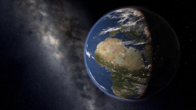
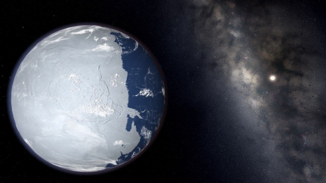
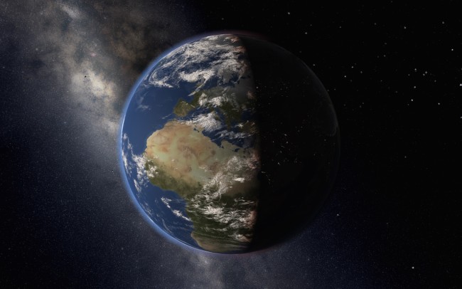
3 Earths with different climates in Universe Sandbox
(from the left: colder Earth, normal Earth, tidally-locked Earth)
Third you can change the parameters of the model itself. What if the heat capacity of the ocean were larger or smaller? What if the heat were transferred less efficiently between land and ocean, or more efficiently between equator and pole? We’ve chosen values that give us realistic behavior for the Earth we live on, but you can see what would happen if it were different. What values are within a realistic range? It’s a sandbox, so you won’t be constrained by that. How sensitive is the simulation to the choice of parameters? Experiment and see.
Oh, and there’s a fourth way of interacting: some of the parameters are indirectly adjusted for you when you change something else about the atmosphere. When you change the concentration of CO2 we’ll change the amount of outgoing infrared energy. When you change the mass of the atmosphere, that new mass will affect the heat capacities. Keep in mind though that this model is designed to capture the behavior of Earth’s climate in realistic scenarios, and the more impossible or extreme you make the inputs the less exact you should expect the outputs to be.
Simulating Complex Systems
As you’ll see from your experiments, you can gain a lot of intuition about complicated subjects by playing around with a simple model. It turns out, this is not so different from what scientists do sometimes to understand the climate system in more detail. It’s much more costly to run a professional climate model with lots of slight tweaks to parameters, just to see what happens. Such sensitivity studies are done nonetheless to verify models. Does it capture some detail of the climate reasonably? How sensitive is the model is to changes in one input or another?
Using computer models to do numerical experiments is not limited to climate science. The climate is but one case where scientists or social scientists study complex systems by prescribing a set of rules for the behavior of the parts and allowing the numerical simulation to reveal what emerges from how they interrelate[3].
The equations that govern our climate models, be they simplified versions or ones with all the complexity our super-computers can handle, come from basic physics. How they interrelate, the sensitivity of the climate to changes – well, you have to run the model to see.
Modeling Climate Change
The direct radiative effect of the additional greenhouse gases humans have been adding to the atmosphere since the start of the industrial age, is only part of the change in energy balance that warms the planet. The feedbacks in the climate system, including albedo feedback, water vapor feedback, and various interactions within clouds (among others) can amplify or dampen the magnitude of the changes in temperature. This is the more difficult part to understand and simulate, and is responsible for much of the range of predictions of different models.
These essential elements of physical climate predictions are inherently the result of interactions between simulated parts, and can best be understood through model experiments. The basic physics of the greenhouse effect is relatively simple, and it doesn’t require a fancy model to conclude that some global warming is to be expected. The interactions between all the parts of the climate system and the feedbacks – that’s more complicated, and requires a model complicated enough to capture them.
In our case, in Universe Sandbox ² we prescribe a relationship between CO2 amount and the outgoing infrared part of the energy balance so that you can experiment with changes in the quantity of greenhouse gases. What feedbacks affect what happens next? Can you determine the climate sensitivity of this model? Are the changes to sea ice cover realistic? This model is pretty simple, but even so it can give you insight into a lot of questions, and hopefully generate even more.
[1] This is why climate scientists run their state-of-the-art models on supercomputers and it still can take weeks to do a single simulation.
[2] This means we’ve divided up the planet into a fixed number of latitudes – however many we want. We pick a number to balance getting enough resolution to show the differences between latitudes, and trying not to make the software so slow as to overwhelm your computer.
[3] A comprehensive and broad introduction to this kind of modeling that includes socio-economic systems can be found in this classic article. Consider also that the greater portion of uncertainty in the climate predictions comes from the scenarios, which are based on socio-economic assumptions about what people will do in the future. Regardless of the scenario, the amount of warming that a given model predicts in response to a fixed increase in CO2 is known as its sensitivity. We are highly confident that the sensitivity of the real climate is somewhere in the range of what the various models predict.
FAQ
How accurate is your climate model?
As you may see by now, models of complicated systems can become as complicated as you like. Making it more complicated doesn’t necessarily give you more accurate results about the simple parts, it just lets you study more aspects of the problem. This model does some simple things quite well, and is also not the right tool to study most of the details of the climate system. You wouldn’t expect great complexity from the “toy model” that runs in real time on your laptop. But you are running a real simulation on your personal computer which can allow you to explore some simple climate features!
Where can I read more about the nitty gritty (equations please!) of the climate calculations you’re using?
The academic journal article reference that is most directly applicable is North and Coakley, 1979.
The scenarios that now appear for potential future climates are the Representative Concentration Pathways used by the Intergovernmental Panel on Climate Change (more details here). The reported CO2 equivalent concentration is tied to the year once a scenario is enabled, and the associated change in outgoing infrared radiation in the scenario is applied directly to the energy balance.
Why can’t I change the albedo when Climate is enabled?
The climate calculations are determining the overall planetary albedo based on how much of the surface is covered by snow and ice. This is what allows for the albedo feedback to be captured by the calculations. If you turn off albedo feedback, the albedo stays the same no matter what you do.
In the simpler case when the Climate component is not enabled you can change the albedo to see how it influences the temperature. The albedo is a number between zero and one (the higher the number the more reflective the planet.) The answer then is as would be expected from this equation:
where T is the temperature, ![]() is the albedo, S is the incoming solar energy,
is the albedo, S is the incoming solar energy, ![]() is the Stefan-Boltzmann constant, and
is the Stefan-Boltzmann constant, and ![]() is the representative overall infrared emissivity, which reflects how much outgoing infrared energy is absorbed and re-emitted by the atmosphere (some of it back towards the surface) on the way.[*]
is the representative overall infrared emissivity, which reflects how much outgoing infrared energy is absorbed and re-emitted by the atmosphere (some of it back towards the surface) on the way.[*]
In a more complicated model, other things would be effecting the albedo as well. Clouds, for example, are even more important than snow and sea ice for the overall global albedo under modern-day Earth conditions.
What’s going on with the clouds?
So far we’re not calculating anything interactively that has to do with the clouds. Most of what you see is visually representative but not simulated. Clouds in the mid-latitudes rotate from West to East, as they do in real life on large-scale. Clouds also fade out when it gets super-hot, super-cold, or super-dry. If you don’t have a giant reservoir of water (the ocean) or it’s totally frozen over and inaccessible to the atmosphere, you won’t have clouds – at least not like the puffy white water clouds we’re used to. And if you make the atmosphere too hot, it will hold more moisture as water vapor and also have fewer clouds (places in the atmosphere where water condenses out into liquid drops).
Later we may make clouds more interactive or let you set some of the parameters.
If you calculate heat diffusion in one equator-pole dimension, how do you decide how to show sea ice and snow at different longitudes?

These are average winter maximum and summer minimum sea ice extents for 1981-2010. See the National Snow and Ice Data Center for more on year-to-year variation, and recent trends.
We make the sea ice edge randomly irregular. Otherwise, based on what we calculate, you’d see smooth concentric circles of ice jumping to higher and lower latitudes. The randomization of the edge makes the sea ice look more “real”, but anyone who has studied Earth’s sea ice will realize that it doesn’t capture the real-life spatial patterns, which do vary geographically depending on basin depth, ocean currents and winds.
What about the snow that forms at higher elevation?
We only calculate one average temperature for each latitude. Then based on the lapse rate, we figure out how high you’d need to be at that latitude in order for it to be cold enough for snow instead of rain. Since we have an elevation map that’s higher resolution than our climate calculations, when we superimpose that snow line onto the elevation map, you can see that higher places are more snow-covered.
Glaciers?
No glaciers yet. We don’t really do anything on such a small scale as a typical glacier. The ice sheets on Greenland and Antarctica are also not modeled at this time in Universe Sandbox. Their greater elevation (from all the ice piled up in real life) usually helps keep them snow covered per our model, as discussed in the last question. But this is why sometimes the edges of those land-masses appear to unfreeze, which is unrealistic. As they lose ice volume in real life, the glacier ice flows out to the ocean, keeping those edges covered.
Because we don’t actually simulate glaciers, there is no change in sea level when Greenland and Antarctica melt. (The sea ice, on the other hand, is a thin skin of ice over the ocean – just a couple of meters thick typically. Because it’s floating on the ocean, melting it doesn’t change sea level anyway.)
Additionally, our elevation model doesn’t have quite the vertical resolution to handle the expected sea level rise of just one or two meters, even though such a change would put a number of important coasts underwater.
When will you simulate life?
Not for a while. For now though you’ll see Earth’s vegetation turn from green to brown when it gets too hot, in case you weren’t keeping an eye on the temperature value or its graph.
* The infrared emissivity is explained in the derivation of the equation.
Scott Manley Simulating the Universe for Fun
Sep 13th
Watch “Astronogamer” Scott Manley run through a series of simulations in Universe Sandbox ² as he discusses a bit of the science behind it all:
Thanks, Scott!
Remember, Universe Sandbox ² is still in alpha, so there are many fixes and improvements that are on their way.
Buy Universe Sandbox ² and get instant access to the alpha on Steam for Windows, Mac, and Linux and pre-order the finished game: http://universesandbox.com/2

